[ad_1]
Object Detection is a helpful tool to have in your coding repository.
It forms the backbone of many fantastic industrial applications. Some of them being self-driving cars, medical imaging and face detection.
In my last post on Object detection, I talked about how Object detection models evolved.
But what good is theory, if we can’t implement it?
This post is about implementing and getting an object detector on our custom dataset of weapons.
The problem we will specifically solve today is that of Instance Segmentation using Mask-RCNN.
Instance Segmentation
Can we create masks for each object in the image? Specifically something like:
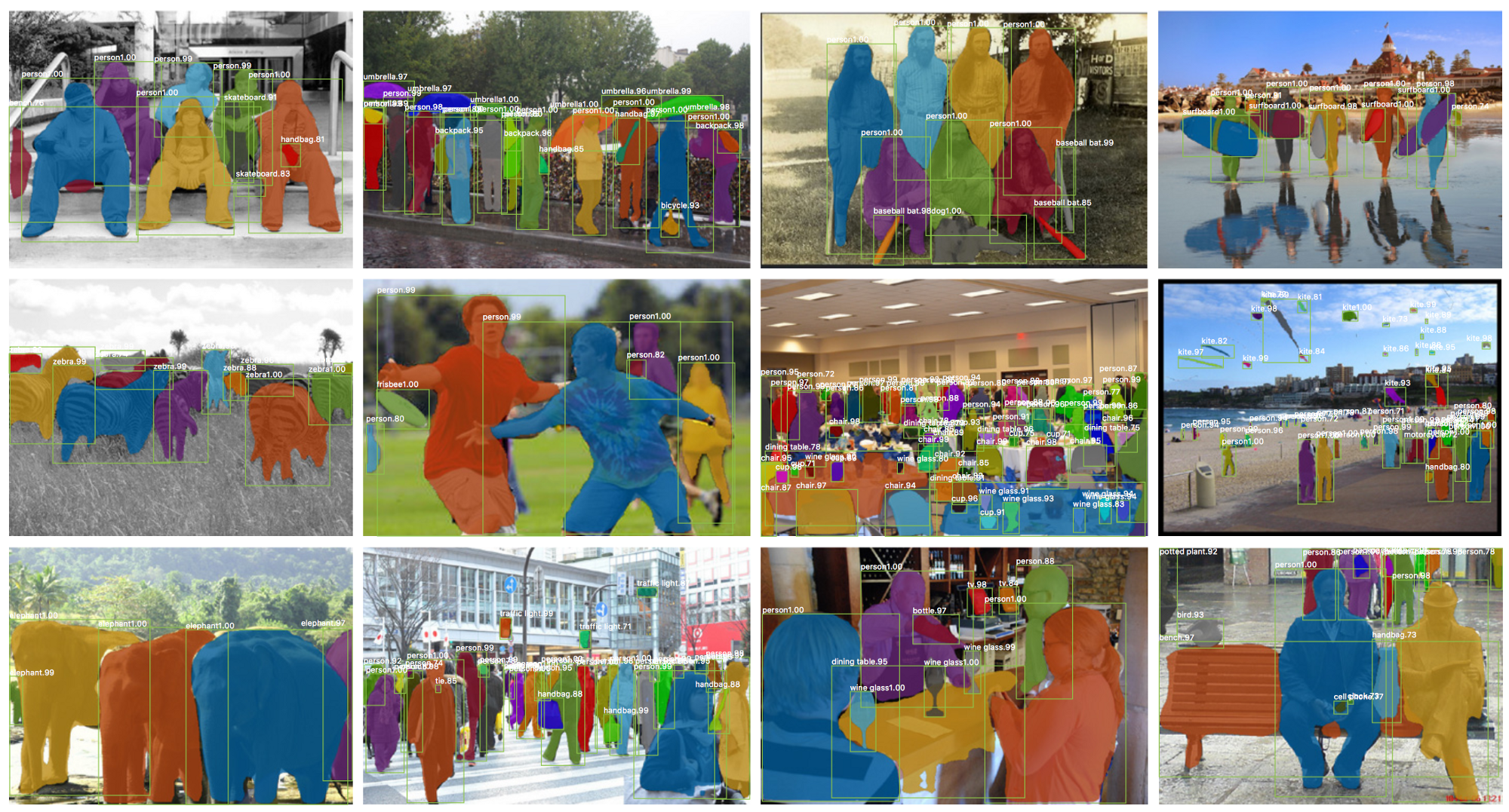
The most common way to solve this problem is by using Mask-RCNN. The architecture of Mask-RCNN looks like below:
](https://mlwhiz.com/images/weapons/1.png)
Essentially, it comprises of:
-
A backbone network like resnet50/resnet101
-
A Region Proposal network
-
ROI-Align layers
-
Two output layers — one to predict masks and one to predict class and bounding box.
There is a lot more to it. If you want to learn more about the theory, read my last post–
Demystifying Object Detection and Instance Segmentation for Data Scientists
This post is mostly going to be about the code.
1. Creating your Custom Dataset for Instance Segmentation

The use case we will be working on is a weapon detector. A weapon detector is something that can be used in conjunction with street cameras as well as CCTV’s to fight crime. So it is pretty nifty.
So, I started with downloading 40 images each of guns and swords from the open image dataset and annotated them using the VIA tool. Now setting up the annotation project in VIA is petty important, so I will try to explain it step by step.
1. Set up VIA
VIA is an annotation tool, using which you can annotate images both bounding boxes as well as masks. I found it as one of the best tools to do annotation as it is online and runs in the browser itself.
To use it, open http://www.robots.ox.ac.uk/~vgg/software/via/via.html
You will see a page like:
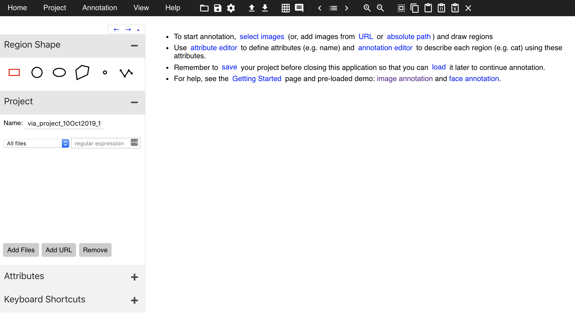
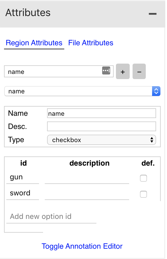
The next thing we want to do is to add the different class names in the region_attributes. Here I have added ‘gun’ and ‘sword’ as per our use case as these are the two distinct targets I want to annotate.
2. Annotate the Images
I have kept all the files in the folder data. Next step is to add the files we want to annotate. We can add files in the data folder using the “Add Files” button in the VIA tool. And start annotating along with labels as shown below after selecting the polyline tool.
3. Download the annotation file
Click on save project on the top menu of the VIA tool.
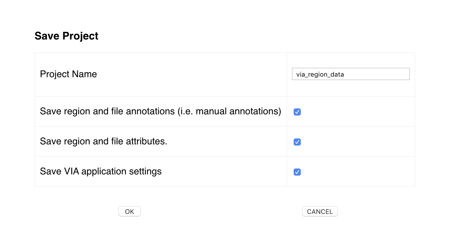
Save file as via_region_data.json by changing the project name field. This will save the annotations in COCO format.
4. Set up the data directory structure
We will need to set up the data directories first so that we can do object detection. In the code below, I am creating a directory structure that is required for the model that we are going to use.
from random import random
import os
from glob import glob
import json
# Path to your images
image_paths = glob("data/*")
#Path to your annotations from VIA tool
annotation_file = 'via_region_data.json'
#clean up the annotations a little
annotations = json.load(open(annotation_file))
cleaned_annotations = {}
for k,v in annotations['_via_img_metadata'].items():
    cleaned_annotations[v['filename']] = v
# create train and validation directories
! mkdir procdata
! mkdir procdata/val
! mkdir procdata/train
train_annotations = {}
valid_annotations = {}
# 20% of images in validation folder
for img in image_paths:
    # Image goes to Validation folder
    if random()<0.2:
        os.system("cp "+ img + " procdata/val/")
        img = img.split("/")[-1]
        valid_annotations[img] = cleaned_annotations[img]
    else:
        os.system("cp "+ img + " procdata/train/")
        img = img.split("/")[-1]
        train_annotations[img] = cleaned_annotations[img]
# put different annotations in different folders
with open('procdata/val/via_region_data.json', 'w') as fp:
    json.dump(valid_annotations, fp)
with open('procdata/train/via_region_data.json', 'w') as fp:
    json.dump(train_annotations, fp)
After running the above code, we will get the data in the below folder structure:
- procdata
     - train
         - img1.jpg
         - img2.jpg
         - via_region_data.json
     - val
         - img3.jpg
         - img4.jpg
         - via_region_data.json
2. Setup the Coding Environment
We will use the code from the matterport/Mask_RCNN GitHub repository. You can start by cloning the repository and installing the required libraries.
git clone https://github.com/matterport/Mask_RCNN
cd Mask_RCNN
pip install -r requirements.txt
Once we are done with installing the dependencies and cloning the repo, we can start with implementing our project.
We make a copy of the samples/balloon directory in Mask_RCNN folder and create a samples/guns_and_swords directory where we will continue our work:
cp -r samples/balloon samples/guns_and_swordsSetting up the Code
We start by renaming and changing balloon.py in the samples/guns_and_swords directory to gns.py. The balloon.py file right now trains for one target. I have extended it to use multiple targets. In this file, we change:
-
balloonconfigtognsConfig -
BalloonDatasettognsDataset: We changed some code here to get the target names from our annotation data and also give multiple targets. -
And some changes in the train function
Showing only the changed gnsConfig here to get you an idea. You can take a look at the whole gns.py code here.
class gnsConfig(Config):
    """Configuration for training on the toy  dataset.
    Derives from the base Config class and overrides some values.
    """
    # Give the configuration a recognizable name
    NAME = "gns"
    # We use a GPU with 16GB memory, which can fit three image.
    # Adjust down if you use a smaller GPU.
    IMAGES_PER_GPU = 3
    # Number of classes (including background)
    NUM_CLASSES = 1 + 2  # Background + sword + gun
    # Number of training steps per epoch
3. Visualizing Images and Masks
Once we are done with changing the gns.py file,we can visualize our masks and images. You can do simply by following this Visualize Dataset.ipynb notebook.
4. Train the MaskRCNN Model with Transfer Learning
To train the maskRCNN model, on the Guns and Swords dataset, we need to run one of the following commands on the command line based on if we want to initialise our model with COCO weights or imagenet weights:
# Train a new model starting from pre-trained COCO weights
 python3 gns.py train — dataset=/path/to/dataset — weights=coco

# Resume training a model that you had trained earlier
 python3 gns.py train — dataset=/path/to/dataset — weights=last

# Train a new model starting from ImageNet weights
 python3 gns.py train — dataset=/path/to/dataset — weights=imagenet
The command with weights=last will resume training from the last epoch. The weights are going to be saved in the logs directory in the Mask_RCNN folder.
This is how the loss looks after our final epoch.

Visualize the losses using Tensorboard
You can take advantage of tensorboard to visualise how your network is performing. Just run:
tensorboard --logdir ~/objectDetection/Mask_RCNN/logs/gns20191010T1234You can get the tensorboard at
https://localhost:6006
Here is how our mask loss looks like:
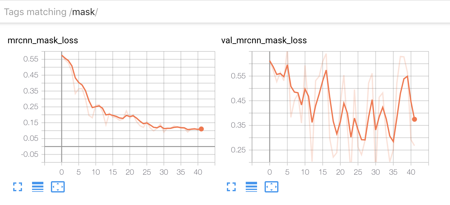
We can see that the validation loss is performing pretty abruptly. This is expected as we only have kept 20 images in the validation set.
5. Prediction on New Images
Predicting a new image is also pretty easy. Just follow the prediction.ipynb notebook for a minimal example using our trained model. Below is the main part of the code.
# Function taken from utils.dataset
def load_image(image_path):
"""Load the specified image and return a [H,W,3] Numpy array.
"""
# Load image
image = skimage.io.imread(image_path)
# If grayscale. Convert to RGB for consistency.
if image.ndim != 3:
image = skimage.color.gray2rgb(image)
# If has an alpha channel, remove it for consistency
if image.shape[-1] == 4:
image = image[..., :3]
return image
# path to image to be predicted
image = load_image("../../../data/2c8ce42709516c79.jpg")
# Run object detection
results = model.detect([image], verbose=1)
# Display results
ax = get_ax(1)
r = results[0]
a = visualize.display_instances(image, r['rois'], r['masks'], r['class_ids'], dataset.class_names, r['scores'], ax=ax,
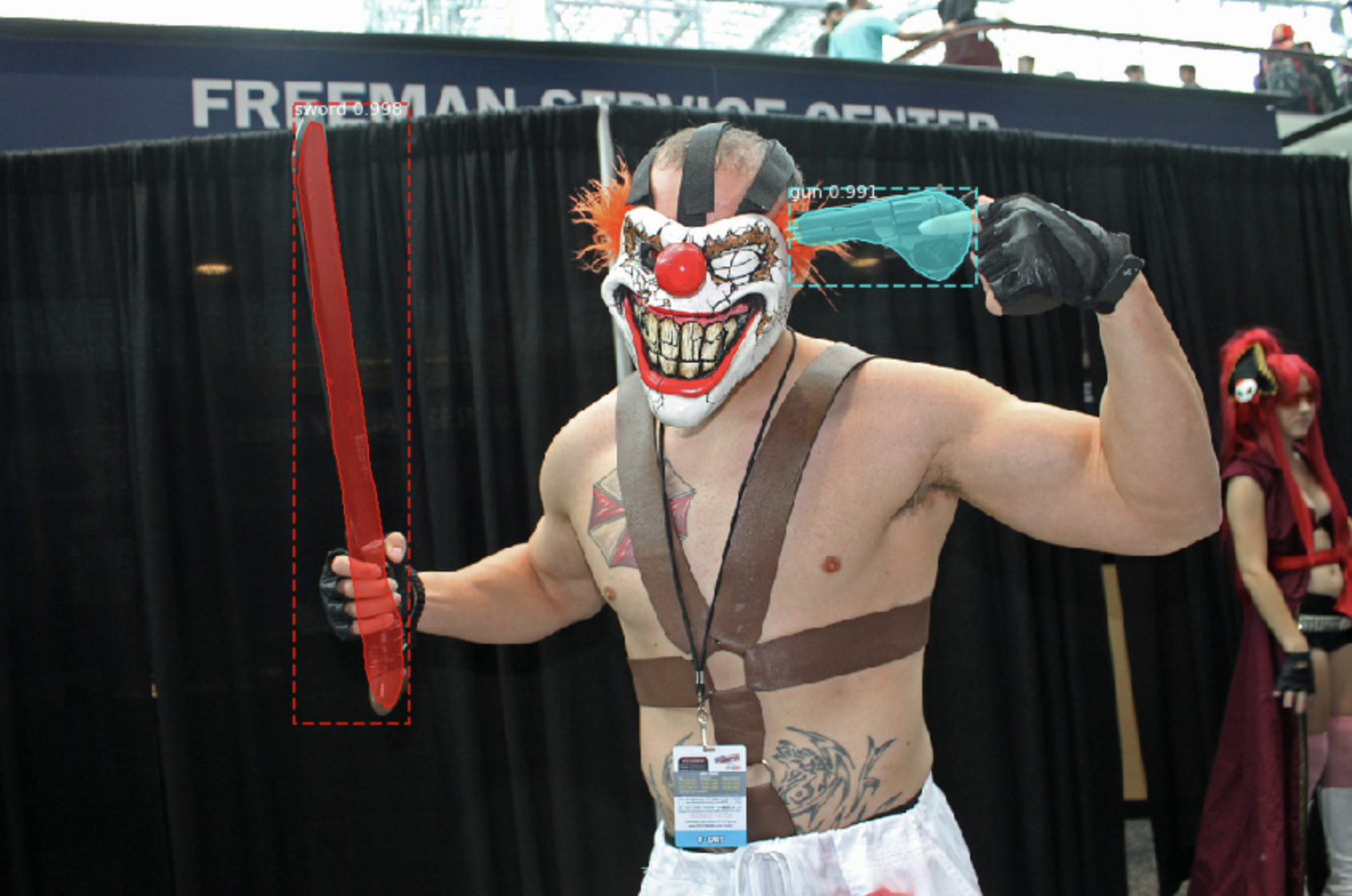
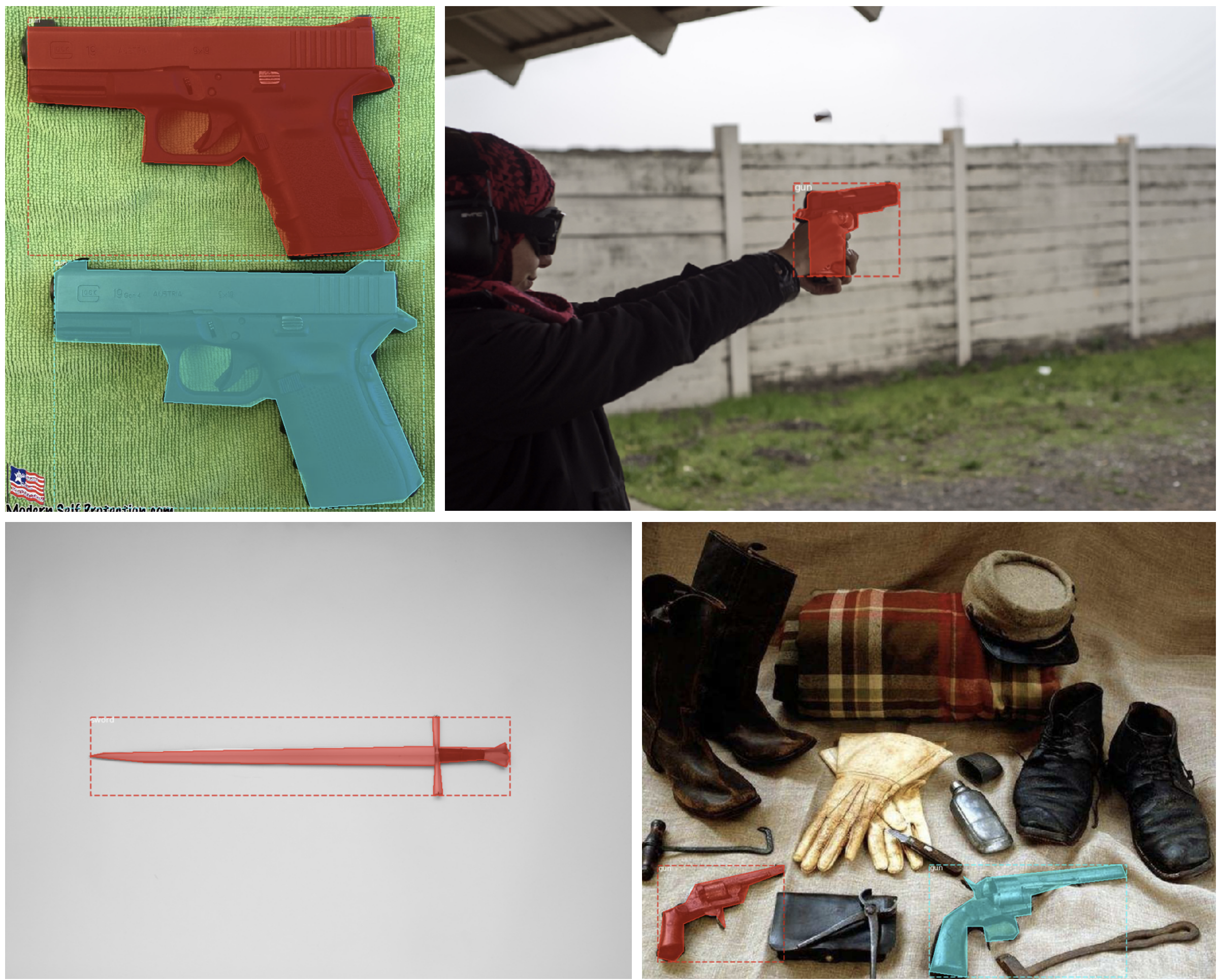
title="Predictions")This is how the result looks for some images in the validation set:
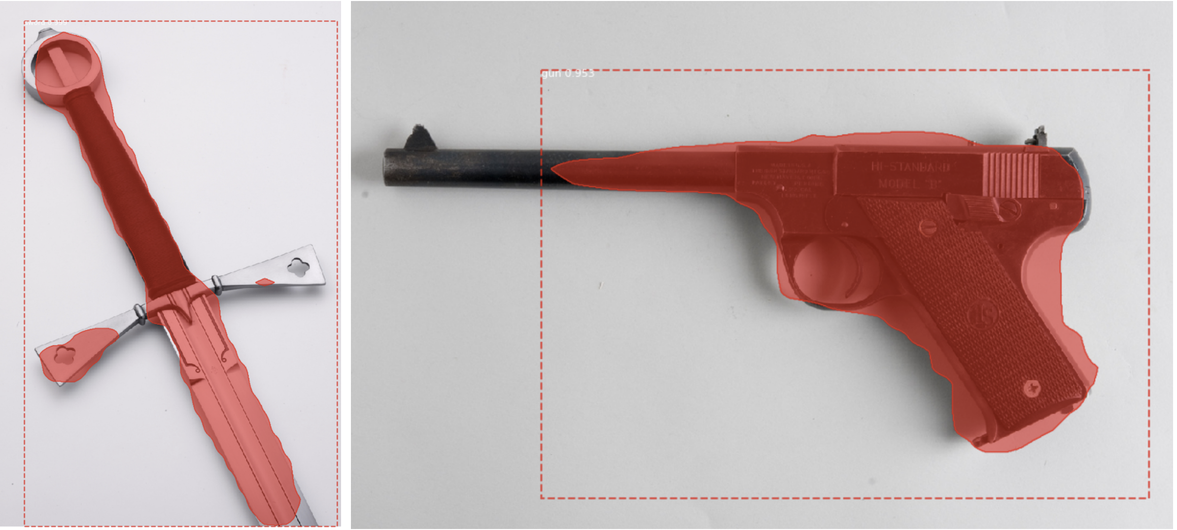
Improvements
The results don’t look very promising and leave a lot to be desired, but that is to be expected because of very less training data(60 images). One can try to do the below things to improve the model performance for this weapon detector.
-
We just trained on 60 images due to time constraints. While we used transfer learning the data is still too less — Annotate more data.
-
Train for more epochs and longer time. See how validation loss and training loss looks like.
-
Change hyperparameters in the mrcnn/config file in the Mask_RCNN directory. For information on what these hyperparameters mean, take a look at my previous post. The main ones you can look at:
# if you want to provide different weights to different losses
LOSS_WEIGHTS ={'rpn_class_loss': 1.0, 'rpn_bbox_loss': 1.0, 'mrcnn_class_loss': 1.0, 'mrcnn_bbox_loss': 1.0, 'mrcnn_mask_loss': 1.0}

# Length of square anchor side in pixels
RPN_ANCHOR_SCALES = (32, 64, 128, 256, 512)

# Ratios of anchors at each cell (width/height)
# A value of 1 represents a square anchor, and 0.5 is a wide anchor
RPN_ANCHOR_RATIOS = [0.5, 1, 2]
Conclusion
In this post, I talked about how to implement Instance segmentation using Mask-RCNN for a custom dataset.
I tried to make the coding part as simple as possible and hope you find the code useful. In the next part of this post, I will deploy this model using a web app. So stay tuned.
You can download the annotated weapons data as well as the code at Github.
If you want to know more about various Object Detection techniques, motion estimation, object tracking in video etc., I would like to recommend this awesome course on Deep Learning in Computer Vision in the Advanced machine learning specialization.
Thanks for the read. I am going to be writing more beginner-friendly posts in the future too. Follow me up at Medium or Subscribe to my blog to be informed about them. As always, I welcome feedback and constructive criticism and can be reached on Twitter @mlwhiz.
Also, a small disclaimer — There might be some affiliate links in this post to relevant resources as sharing knowledge is never a bad idea.
[ad_2]
Source link
Emprendedor en el sector de los videojuegos, tecnologica y educación. + de 20 años en videojuegos. CEO de Hydra Interactive. Fundador de Devsfromspains.

![Buildbox Free - How To Make 2D Platformer Game [PART 1]](https://e928cfdc7rs.exactdn.com/info/uploads/sites/3/2020/01/Buildbox-Free-How-To-Make-2D-Platformer-Game-PART-150x150.jpg?strip=all)

