Prostate Cancer Detection using Deep Convolutional Neural Networks

Data

A cohort of 427 consecutive patients with a PI-RADS score of 3 or higher who underwent biopsy were included. Out of 427 patients, 175 patients had clinically significant prostate cancer and 252 patients did not. A total of 5,832 2D slices of each DWI sequence (e.g., b0) which contained prostate gland were used as our dataset. We set the patient with Gleason score higher than or equal to 7 (International Society of Uropatholgists grade group (GG >= 2) as the patient with a clinically significant prostate cancer and patient with Gleason score lower than or equal to 6 (GG = 1) or with no cancer (GG = 0) as the patient without a clinically significant prostate cancer.

MRI Acquisition

The DWI data was acquired between January 2014 to July 2017 using a Philips Achieva 3T whole body unit MR imaging scanner. The transverse plane of DWI sequences was obtained using a single-slot spin-echo echo-planar imaging sequence with four b values (0, 100, 400, and 1000s mm({}^{-2})), repetition time (TR) 5000~7000 ms, echo time (TE) 61ms, slice thickness 3mm, field of view (FOV) 240 mm (times ) 240 mm and matrix of 140 (times ) 140.

DWI is an MRI sequence which measures the sensitivity of tissue to Brownian motion and it has been found to be a promising imaging technique for PCa detection³². The DWI image is usually generated with different b values (0, 100, 400, and 1000s mm({}^{-2})) which generates various signal intensities representing the amount of water diffusion in the tissue and can be used to estimate ADC and compute high b-value images (b1600)³³.

In order to use DWI images as input to our deep learning network, we resized all of the DWI slices into 144 (times ) 144 pixels, and center cropped them with 66 (times ) 66 pixels such that the prostate was covered. The CNNs were modified to feed DWI data with 6 channels (ADC, b0, b100, b400, b1000, and b1600) instead of images with 3 channels (red, green and blue.)

Training, validation, and test sets

We separated 427 patients DWI images into three different sets, the training set with 271 patients (3,692 slices), the validation set with 48 patients (654 slices), and the test set with 108 patients (1,486 slices) where the training/validation/test ratio was 64%, 11%, 25%. The separation procedure of the dataset was as follows. First, we separated the dataset into two sets, the training/validation set as 75% and the test set as 25% to maintain a reasonable sample size for the test set. Second, we separated the training/validation set into two sets with training set as 85% of training/validation set and the validation set as 15% of training/validation set (Table 1). The ratios between the PCa patients and non PCa patients were kept roughly similar throughout the data sets.

Data preprocessing

All of DWI images in the dataset were normalized across the entire dataset using the following function.

where ({X}_{i}) is the pixels in an individual MRI slice, (mu ) is the mean of the dataset, std is the standard deviation of the dataset, and ({X}_{i{rm{_}}normalized}) is the normalized individual MRI slice.

Pipeline

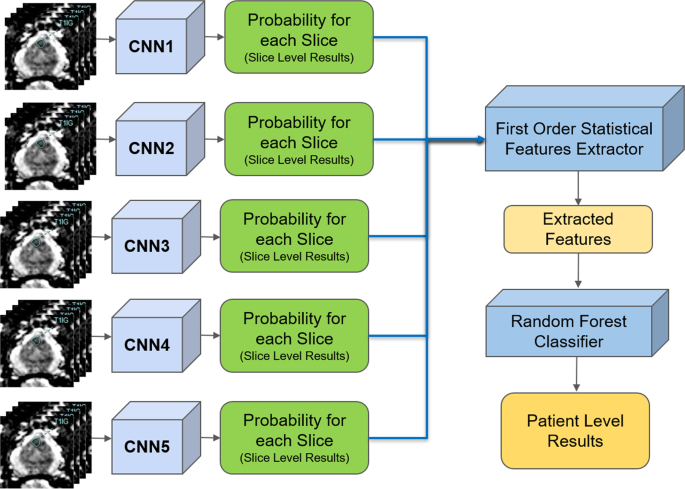
The proposed pipeline consists of three stages. In the first stage, each DWI slice is classified using five individually trained CNNs models. In the second stage, first-order statistical features (e.g., mean, standard deviation, median, etc.) are extracted from the probability sets of CNNs outputs, and important features are selected through a decision tree-based feature selector. In the last stage, a Random Forest classifier is used to classify patients into groups with and without PCa using these first order statistical features. The Random Forest classifier was trained and fine-tuned by the features extracted from the validation set with 10 fold cross-validation method. Figure 1 shows the block diagram of the proposed pipeline.

Block diagram of the proposed pipeline for prostate cancer detection. The inputs to each CNN are 66 (times ) 66 (times ) 6 (ADC, b0, b100, b400, b1000, b1600) MRI slices. The output is the slice level and patient level results.

ResNet

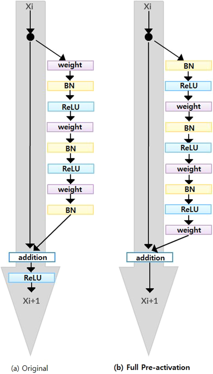
Since ResNet architecture has shown promising performance in multiple computer vision tasks¹⁷, we chose it as our base architecture for this research. Each Residual Block consists of convolutional layers²¹ and identity shortcut connection¹⁷ that skips those layers, and their outcomes are added at the end, as shown in Figure 2-a. When input and output dimensions are the same, the identity shortcuts, denoted by x, can be directly applied. The following formula shows the identity mapping process.

where (F(x,{W}_{i})) is the output from convolutional layers and x is the input. When the dimension of input is not the same as that of the output (e.g., at the end of the Residual Block), the linear projection ({W}_{s}) changes the dimension of the input to be same as that of the output which is defined as:

The structural difference between original residual network and fully pre-activated residual network.

To improve the performance of the architecture, we implemented a fully pre-activated residual network³⁴. In the original ResNet, batch normalization and ReLU activation layers were followed after the convolution layer, but in pre-activation ResNet, batch normalization and ReLU activation layers comes before the convolution layers. The advantage of this structure is that the gradient of a layer does not vanish even when the weights are arbitrarily small³⁴. Instead of 2-layer deep ResNet block, we implemented a 3-layer deep “bottleneck” building block since it significantly reduces training time without sacrificing the performance¹⁷ (Figure 2-b).

CNNs architecture and training

A 41 layers deep ResNet was created for the slice-level classification. The architecture is composed of 2D convolutional layers with a 7 (times ) 7 filter followed by a 3 (times ) 3 Max pooling layer and residual blocks (Res Block). The depth of 41 layers were found to be optimal through hyper-parameter fine-tuning procedure using the validation set. Since the input images were small (66 (times ) 66 pixels) and the tumorous regions were even smaller (e.g., 4 (times ) 3 pixels), additional ResNet blocks or deeper networks were needed. The first ResNet Block (ResNet Block1 in Table 2) is 3-layer bottleneck blocks with 2D CNN layers with filter sizes 64, 64 and 256 which is stacked 4 times. The second ResNet Block (ResNet Block2 in Table 2) is 3-layer bottleneck blocks with 2D CNN layers with filter sizes 128, 128, and 512 which is stacked 9 times. 2 (times ) 2 2D Average Pooling, Dropout layer, and 2D Fully connected Layer with 1000 nodes for two probabilistic outputs are followed by the end of Res Blocks. Table 2 shows the overview of the proposed CNNs architecture.

Stochastic Gradient Decent³⁵ was used as the optimizer with the initial learning rate of 0.001, and it was reduced by a factor of 10 when the model stopped improving after iterations. The model was trained with the batch size set to 8. Dropout rate was set to 0.90. We used a weight decay of 0.000001 and a momentum of 0.90. Since the dataset is extremely unbalanced, binary cross entropy³⁶ was used as the loss function.

Stacked generalization

Due to the randomness in training CNNs (for instance, at the beginning of training CNNs, weights are set to arbitrary random numbers), each CNN may be different despite identical set of hyper-parameters and input datasets. This means each CNN may capture different features for the patient-level classification. Stacked generalization³⁷ is an ensemble technique that trains multiple classifiers with the same dataset and makes a final prediction using a combination of individual classifiers’ predictions. Stacked generalization typically yields better classification performance compared to a single classifier³⁷. We implemented a simple stacked generalization method using five CNNs. The number of stacked CNNs was selected based on the best performance and increasing the number of CNNs did not show improvement on the patient-level performance. Since there is a limited sample size for patient level (48 patients for validation, which was used to train Random Forest classifier for patient-level detection), increasing the number of CNNs, which leads to an increased number of patient-level features (as discussed in the next section), increases the likelihood of overfitting and hence, decreases the model’s robustness³⁸. All the slice-level probabilities generated by the five CNNs were fed into a first-order statistical features extractor to generate one set of features for each patient. In the proposed pipeline, the patient-level performance significantly improved (2-tailed P = 0.048) using five CNNs compared to a single CNN (AUC: 0.84, CI: 0.76–0.91, vs. AUC: 0.71, CI: 0.61–0.81).

First order statistical feature extraction

Let ({p}_{ij}) and ({n}_{ij}) be the probabilities of a MRI slice associated with PCa and non PCa, respectively, where (i) represents one of five individually trained CNNs and (j) represents each MRI slice of a patient. Each CNN produces two probability sets, ({P}_{i}=left{{p}_{i1},…,{p}_{iN}right}) and ({N}_{i}=left{{n}_{i1},…,{n}_{iN}right}) where (N) is the total number of MRI slices for each patient. Within the probability sets, top five probabilities which are higher than 0.74 were selected ((acute{{P}_{i}}) and (acute{{N}_{i}})). This was done to ensure less relevant probabilities at slice level were not used for patient-level classification. The probability cutoff of 0.74 was selected by grid-search using the validation set. Next, from the new probability sets, (acute{{P}_{i}}) and (acute{{N}_{i}}), the first-order statistical features set, ({F}_{i}={{f}_{i1},…{f}_{iK}}) where K represents the total number of statistical features, were extracted for each patient. Next, the important features, (acute{{F}_{i}}) were selected by a decision tree-based feature selector³⁹. The final feature set was constructed by combining important features, (acute{{F}_{i}}), for all five CNNs where (F={acute{{F}_{1}},…acute{{F}_{5}}}).

We extracted nine first-order features which are the mean, standard deviation, variance, median, sum, minimum (only from non PCa class), maximum (only from PCa class), skewness⁴⁰, kurtosis⁴⁰, and range from the minimum to maximum from each probability set. This produced 90 features for each patient (9 features for PCa and 9 features for non PCa class for each CNN). We selected 26 best features using the decision tree-based feature selector³⁹. The decision tree based-feature selector was fine-tuned and trained with 10 fold cross-validation method using the validation set (Fig. 3).

Block diagram of the proposed first-order statistical feature extractor. PCa Set: probabilistic output set from each CNN which is associated with PCa class. Non PCa Set: probabilistic output set from each CNN which is associated with non PCa class.

Once first-order statistical features were extracted for each patient, a Random Forest classifier^30,31 was trained using the validation set and tested on the test set for patient-level classification.

Computational time

The CNNs were trained using one Nvidia Titan X GPU, 8 cores Intel i7 CPU and 32 GB memory. It took 6 hours to train all five CNNs with up to 100 iterations, less than 10 seconds to train the Random Forest classifier, and less than 1 minute to test all 108 patients.

Ethics approval and consent to participate

The Sunnybrook Health Sciences Centre Research Ethics Boards approved this retrospective single institution study and waived the requirement for informed consent.