Neural Network Fundamentals

Ever thought about learning Artificial Intelligence? In this series of articles we will share with you some of the Neural Network Fundamentals that will allow you to start your journey

In this first post of a series of three, we will talk about one of the most important branches of Machine Learning and Artificial Intelligence, Neural Networks. We will approach this topic from scratch, starting with the history of neural networks, their basic concepts, we will go into the mathematics involved in them and we will implement an example of Neural Networks from scratch to recognize certain types of patterns in images.

Introduction Neural Network Fundamentals

Neural networks are part of the field of Artificial Intelligence. First of all, it is worth mentioning that 25 years ago practically nobody knew what the Internet was or what it meant, as you can see in this video from the Today Show in 1994. Neural networks were invented in the 60’s, what happened then?

A bit of history

In 1994, computers had very limited capabilities. This is the main reason why neural networks were not used at that time, despite being invented decades earlier. Computers did not yet have the computational capacity. Nor did they have the data processing and storage capacity to work with neural networks. However, the 1970s and 1980s are characterized by futuristic movies with robots and machines taking control.

In Terminator or Blade Runner, where it is clear that the concept of intelligent machines was already latent at that time. Unfortunately, in the following decades, this interest waned. Although there was extensive research in universities on Artificial Intelligence. In fact, it was thought that the world of neural networks came to an end. It was a nice theory but with no possible practical application.

However, the growth in all aspects of computers has been exponential since that time.

Deep Learning

Surely you have seen many times an image like the following one:

Deep Learning with input arrows on the left, a certain brain processes them and from that moment on they are transformed into digital data:

The father of the Deep Learning concept was the British Geoffrey Hinton. He did research on Deep Learning in the 1980s, currently works at Google, and many of the things we will talk about come from Geoffrey Hinton’s nomenclature. The main idea behind the concept of Deep Learning is to look at the human brain and take inspiration from it to try to computationally reproduce its behavior. So, if what we are trying to do is to mimic the human brain, we have to bring certain elements of neuroscience to the computer. Let’s see how we do this.

The human neuron

In the following image we can observe human neurons under the microscope.

In it we can observe a kind of mass or body more or less round. In addition, we see a nucleus or center, and a series of branches that extend. In the brain, more or less, we have about one hundred billion neurons. Therefore, what we are trying to do is to transfer the behavior of the human brain to a machine, taking into account that the knowledge we have of the human brain is still very limited.

Neural networks

So let’s see how we go from the neurons in the human brain to form a neural network in a machine that simulates its behavior.

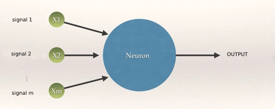
The Artificial Neuron

Artificial neurons are modeled in such a way that they mimic the behavior of a brain neuron. They will have branches and a nucleus or node. There will be input branches to the node, which will be the inputs to the neuron from other neurons. This information will be processed in a node, and output information will be generated and transmitted by the output branches to other neurons. We can think of the connections between artificial neurons as the synapses of neurons in the brain. The image of a typical artificial neuron is as follows.

The neural network

In the following image we can see some models of neural networks.

We see that the output branches of some neurons are the input branches of others, and so on. But we see a couple of differences between the layers. The neurons in red have no input branches. They are information that we are going to give to the neurons “from the outside,” or “initial stimulus.” We also see that the blue neurons have output branches that are not connected to other neurons. They are the output information of the neural network or “final stimulus”. Depending on the number of hidden layers (yellow) we can speak of a simple or deep neural network.

Output values and weights of neural networks

Output values can be continuous, such as the price of a particular purchase. They can also be binary, such as whether or not a person will suffer from a disease. Or they can be a category, such as the brand of car that will sell the most next year. In this context, the binary case is a particular case where we have two categories.

In order to carry out the processing, each synapse will be assigned a value or weight. They are equivalent to the “strength” of the signal transmitted by each synapse. The adjustment of these weights in order to have a neural network that does what we want is fundamental. We will discuss this at length when we talk about neural network training. We will look at methods for adjusting these weights, such as gradient descent and backpropagation. Let’s then look at how information is processed within each neuron.

Information processing of an artificial neuron

The input signals we see in the image above are independent variables, input parameters that will be processed by the body of the artificial neuron to finally propagate the result to an output signal. Therefore, the transmission arrows from the inputs to the nucleus of the neuron would play the role of the synapse of the brain neurons. We then have a layer of input neurons, a layer of hidden neurons (in the image one) and a layer of output neurons (one or more).

All the independent variables in the input layer belong to a single observation, a single sample, “a single record in the database”.

The core of the neuron is where the input signals and weights are processed. One of the ways is to multiply each input signal by its weight and add it all up, i.e. make a linear combination of the weights of the connections and the inputs.

w_0 x_0 + w_1 x_1 + w_2 x_2 + … + w_N x_mw0x0+w1x1+w2x2+…+wNxm

as we see in the first step of the following image. Subsequently, a certain activation function is applied to the result of the first step, and the final result is propagated to the output, third step of the image.

y = \phi(w_0 x_0 + w_1 x_1 + w_2 x_2 + … + w_N x_m)

y=ϕ(w0x0+w1x1+w2x2+…+wNxm)

Information processing in a neuron

Let’s take a look at the four most typical activation functions that are commonly used.

Activation functions

First the linear combination of weights and inputs is calculated. The activation functions are simply the way to transmit this information through the output connections. We may be interested in transmitting this information unmodified, so we would simply use the identity function. In other cases, we may not want any information to be transmitted. That is to say, to transmit a zero at the outputs of the neuron.

In general, activation functions are used to give a “non-linearity” to the model and make the network capable of solving more complex problems. If all activation functions were linear, the resulting network would be equivalent to a network without hidden layers.

We are going to see the four families of activation functions most commonly used in neural networks.

Threshold function

As we can see in the figure below, on the x-axis is represented the already weighted value of the inputs and their respective weights, and on the y-axis we have the value of the step function. This function propagates a 0 if the value of x is negative, or a 1 if it is positive. There are no intermediate cases, and it serves to classify very strictly. It is the most rigid function.

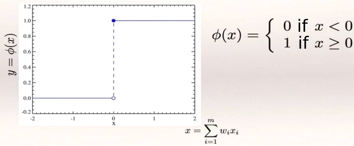
Step function

Sigmoid function

As in the step function, there is a division between negative and positive values of x, but the sigmoid function is not so strict, the change is made smoothly. It is used in logistic regression, one of the most used techniques in Machine Learning. As we see in the figure below, the function has no edges, it is smoother (in mathematical terms, it is derivable). The more positive the value of x the closer we get to 1 and conversely, the more negative x the closer we get to 0.

Sigmoid function

This function is very useful in the final output layer at the end of the neural network, not only to classify with categorical values, but also to try to predict the probabilities of belonging to each category, where we know that the probability of an impossible event is 0 and that of a safe event is 1.

Rectifier function (ReLU)

We have again in this function an edge. We see in the figure below that its value is 0 for any negative value of x.  If x is positive the function returns the value of x itself. Therefore, all those entries that once weighted have a negative value are ignored and we are left with the exact value of the positive ones. We also see that, unlike the previous ones, the values are not restricted to values between 0 and 1.

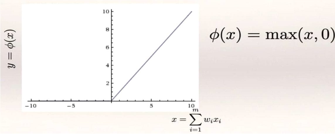
Rectifier function

Hyperbolic tangent function

This function is very similar to the sigmoid function, but in this case, as we see in the figure below, it does not start at 0 and end at 1, but starts at -1 and ends at 1.

Hyperbolic tangent function

Neural network configuration

We already have the basic ingredients to configure a neural network. An input neuron layer, where we will pass information to the network as stimuli, a hidden neuron layer, which will be in charge of processing the information provided by the input layer, and an output layer that will process the information provided by the hidden layer to obtain the final result of the neural network for a specific input. A possible configuration could be as shown in the figure below.

Example of a neural network configuration

We have done the weighting of the output signals with a linear combination, in the hidden layer we use a rectifier function and in the output layer we use a sigmoid function. You can use in your neural networks any other type of function that best fits the problem to be solved, this is just an example.

The choice of one activation function or another will depend on several factors. One of them is the range of values that we want in the output of the neuron. If there is no restriction on the range, we will use the identity function that will propagate the input value to the output. If the constraint is only that the output value must be positive, with no quantity limit, we will choose a rectifier function. We may be interested in a binary output 1 and 0 for sorting, so we choose, for example, the step function.  We may use a learning algorithm that makes use of derivatives. Then we will use activation functions where the derivative is defined over the whole interval.

For example the sigmoidal or the hyperbolic tangent, taking into account that they are more computationally expensive.

The cost function

During training, we have the input values and we know what their respective outputs are. What we want is to adjust the weights so that the neural network learns, and the output values of the network are as close as possible to the real known values. Let’s see with a small example the whole process.

Suppose we want to build a neural network that, once trained, predicts the price of a house. To do so, we collect the following data on thousands of houses:

• Surface
• Age of the house
• Number of bedrooms
• Distance to the city

We will have thousands of records in a database, with information about the houses and their current value. The weights of the different connections between neurons will be initialized in some way (we will see how). We will start to introduce in the network the records corresponding to each house and, for each one of them, we will obtain an output value that generally will not be equal to the real values of the price of the houses.

The cost function is a function that measures, in a sense, the “difference” between the output value and the present value. In this example we will use the mean square error. Of course, it can be a more complex function.

We feed the neural network in different iterations with the same training data we have, and in each iteration we try to minimize the cost function. That is to say that the difference between the output values and the real ones is smaller and smaller. As the input data are what they are, we can only achieve this by adjusting the weights of the connections between neurons at the end of each iteration.

Actual value – prediction

Summarizing, at the end of each iteration, for each floor an output value (prediction) will be obtained from the neural network. This value will differ by an amount with respect to the actual value measured by the cost function.

Now, we update the weights of the neural connections and feed back the neural network with the initial data of the floors. The process is repeated again and the weights are adjusted so that the cost function becomes smaller and smaller.

One way to calculate the cost function is as shown in the figure below. We calculate the square of the difference between the output and actual value (avoiding negative values) of each house. Then we add up the value for all the houses and divide by 2 (we will address the math in subsequent posts).

Values for the cost function

Once the process is finished, we will have a trained neural network ready to predict the price of a house by supplying the house data. In general, the network will make excellent predictions for the data we have used to train it. But to evaluate the prediction quality of the neural network it is necessary to use data that has not been used to optimize the weights of the network connections.

Conclusion: Neural Network Fundamentals

We already have the basic notions of what a neural network is. With all the information we have about a given problem, in our case apartment prices, we build a neural network that learns from that data. Finally, the network will be able to predict correctly when we ask for data that the network has never seen.

In this post we have seen some simple mathematical concepts, such as activation functions. In the next one, we will really get into the mathematics behind neural networks. The activation functions of the neurons we have seen are very important. Their correct choice will provide us with a neural network that makes good predictions. Basically, the activation functions we have seen return either a value between zero and one, or the same input value if it is positive (rectifier).

In the next post we will see how to adjust the weights of the neural network connections. To start working with examples of neural networks, it is not necessary to know the mathematics on which they are based. But there are advantages to knowing the mathematics behind any machine learning algorithm. When the results are not good enough, we can get ideas on how to improve performance. If we don’t have this mathematical basis, we will have no choice but to settle for the result we have.

We will see that the problem of adjusting weights “by brute force”, i.e. trying all possibilities and keeping the best one, is in practice impossible since it would take millions of years of computation to find the best solution. However, mathematics allows us to find this solution in a reasonably short time.